既然是重新熟悉 Spark,不免俗的要來試著自己寫寫 Spark application,以前都是寫 Scala,但我想現在寫 Python 的人佔大宗所以之後就用 pyspark 來寫 applicatoin 吧!
Environment
來準備一下環境吧,Spark 可 run 在以下的環境:
Spark runs on Java 8/11/17, Scala 2.12/2.13, Python 3.8+
Java
Java 我選擇版本 Java 17,因為我是 mac 所以用 Homebrew 可以很輕鬆寫意的安裝 Java 17,
brew install openjdk@17若要讓 mac os 用這個 java,建議在以下資料夾下建立 soft link。
sudo ln -sfn /opt/homebrew/opt/openjdk@17/libexec/openjdk.jdk /Library/Java/JavaVirtualMachines/openjdk-17.jdk
然後別忘了要在你的環境變數 PATH 中加入 java 路徑,
echo 'export PATH="/opt/homebrew/opt/openjdk@17/bin:$PATH"' >> ~/.zshrc我是用 oh-my-zsh,所以我的 profile 名稱為 zshrc
最後確認 Java 是否安裝成功。
~ ❯ java --version
openjdk 17.0.15 2025-04-15
OpenJDK Runtime Environment Homebrew (build 17.0.15+0)
OpenJDK 64-Bit Server VM Homebrew (build 17.0.15+0, mixed mode, sharing)
Python
然後是 Python,我選擇使用用 conda 建了個 Python 3.12 的環境,然後安裝 pyspark,Spark 版本我們選擇 3.5.5,
conda create -n spark-cluster python=3.12
conda activate spark-cluster
pip install pyspark==3.5.5 matplotlib==3.10.0 pandas==2.2.3
然後建一個有以下目錄結構的 python project
apps/
data/input/
data/output/
README.md
requirements.txt
Data
今天這個 application 是用 MovieLens 的資料來做一下電影評分統計,資料我們用 recommended for new research,這份資料的電影評分數有 32,000,205 筆,
下載地方如下圖標記的位置,
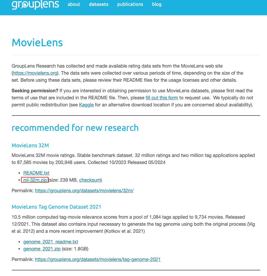
你也可以直接點這個 連結 下載,
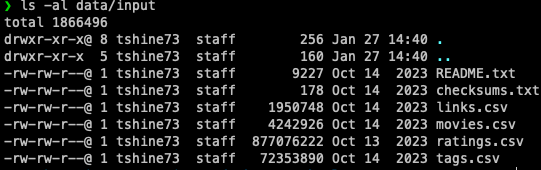
下載完成後,在 data/input/ 這個資料夾 unzip,完成後如下圖。
主程式
首先用以下程式建立一個 spark session,
import os

from pyspark.sql import SparkSession
from pyspark.sql.functions import avg, count, round, col, lit
import time

def init():
    spark = SparkSession.builder.getOrCreate()
    return spark
取得 spark session 後,再來可以用以下程式讀取 MovieLens CSV 然後 show 幾筆看一下,
spark = init()
ratings_file = os.path.join(DATA_INPUT_PATH, "ratings_sample.csv")
rating_df = spark.read.option("header", True).csv(ratings_file)
rating_df.show()
+------+-------+------+---------+
|userId|movieId|rating|timestamp|
+------+-------+------+---------+
| 1| 17| 4.0|944249077|
| 1| 25| 1.0|944250228|
| 1| 29| 2.0|943230976|
| 1| 30| 5.0|944249077|
| 1| 32| 5.0|943228858|
| 1| 34| 2.0|943228491|
| 1| 36| 1.0|944249008|
| 1| 80| 5.0|944248943|
| 1| 110| 3.0|943231119|
| 1| 111| 5.0|944249008|
| 1| 161| 1.0|943231162|
| 1| 166| 5.0|943228442|
| 1| 176| 4.0|944079496|
| 1| 223| 3.0|944082810|
| 1| 232| 5.0|943228442|
| 1| 260| 5.0|943228696|
| 1| 302| 4.0|944253272|
| 1| 306| 5.0|944248888|
| 1| 307| 5.0|944253207|
| 1| 322| 4.0|944053801|
+------+-------+------+---------+
only showing top 20 rows再來可以用 movieId 統計一下平均評分,
average_rating = rating_df.groupBy("movieId").agg(round(avg("rating"), 1).alias("average_rating"))
average_rating.show()
+-------+--------------+
|movieId|average_rating|
+-------+--------------+
| 1090| 3.9|
| 296| 4.2|
| 3210| 3.7|
| 2294| 3.2|
| 88140| 3.5|
| 158813| 3.0|
| 48738| 3.8|
| 115713| 4.0|
| 829| 2.7|
| 2088| 2.6|
| 3606| 3.9|
| 5325| 3.7|
| 89864| 3.7|
| 2162| 2.5|
| 3959| 3.7|
| 2069| 3.8|
| 85022| 2.7|
| 2136| 2.8|
| 27317| 3.6|
| 4821| 3.2|
+-------+--------------+
only showing top 20 rows接下來我們可以把 movie 的資訊 join 回去,
joined_df = average_rating.join(movie_df, on="movieId") \
        .orderBy(col("average_rating").desc(), col("title").asc())
joined_df.show()
+-------+--------------+--------------------+------------------+
|movieId|average_rating| title| genres|
+-------+--------------+--------------------+------------------+
| 160513| 5.0|$uperthief: Insid...|(no genres listed)|
| 268482| 5.0|'Tis the Season t...| Comedy|Romance|
| 290978| 5.0| 1 Message (2011)| Drama|
| 183647| 5.0|11 September Vrag...| Documentary|
| 266682| 5.0|12 Dog Days Till ...| Children|
| 291268| 5.0| 1500 Steps (2014)| Drama|
| 225429| 5.0|1964: Brazil Betw...| Documentary|
| 180409| 5.0|1984 Revolution (...| Documentary|
| 143422| 5.0| 2 (2007)| Drama|
| 224445| 5.0|2 Years of Love (...| Comedy|Romance|
| 260057| 5.0|24 Hour Comic (2017)| Documentary|
| 200086| 5.0|2BPerfectlyHonest...|(no genres listed)|
| 176709| 5.0| 2nd Serve (2013)| Comedy|Drama|
| 137329| 5.0| 3 of a Kind (2012)|(no genres listed)|
| 137313| 5.0| 37 (2014)|(no genres listed)|
| 253946| 5.0| 48 Below (2012)| Adventure|
| 137805| 5.0|5 Hour Friends (2...|(no genres listed)|
| 188925| 5.0|8 Murders a Day (...|(no genres listed)|
| 170429| 5.0|9 Dalmuir West (1...| Documentary|
| 137849| 5.0| 9 Full Moons (2013)| Romance|
+-------+--------------+--------------------+------------------+
only showing top 20 rows在來我們可以看一下各平均分數下的電影數統計,
total = average_rating.count()
movie_rating_count = average_rating.groupBy("average_rating").agg(count("*").alias("count_movies")) \
        .withColumn("percentage", round((col("count_movies") / lit(total)) * 100, 2)) \
        .orderBy("average_rating", ascending=False)
movie_rating_count.show()
+--------------+------------+----------+
|average_rating|count_movies|percentage|
+--------------+------------+----------+
| 5.0| 1445| 1.71|
| 4.9| 2| 0.0|
| 4.8| 72| 0.09|
| 4.7| 26| 0.03|
| 4.6| 8| 0.01|
| 4.5| 974| 1.15|
| 4.4| 57| 0.07|
| 4.3| 563| 0.67|
| 4.2| 283| 0.34|
| 4.1| 425| 0.5|
| 4.0| 3736| 4.42|
| 3.9| 1286| 1.52|
| 3.8| 3228| 3.82|
| 3.7| 2700| 3.2|
| 3.6| 3152| 3.73|
| 3.5| 8040| 9.52|
| 3.4| 3668| 4.34|
| 3.3| 5819| 6.89|
| 3.2| 3822| 4.53|
| 3.1| 3554| 4.21|
+--------------+------------+----------+最後可以用 matplotlib 來畫張圖看會比較有感,
import matplotlib.pyplot as plt
import numpy as np

movie_rating_count.toPandas().plot.line(x='average_rating', y='percentage', xticks=np.arange(0.5, 5, step=0.5))
plt.show()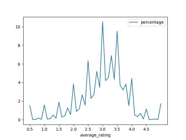
看起來大多數的電影評分都是落在 3~4 之間 XDD
最後提供完整主程式,命名為 main.py 後並放至 app 資料夾底下,
import os
import time

import matplotlib.pyplot as plt
import numpy as np
from pyspark.sql import SparkSession
from pyspark.sql.functions import avg, count, round, col, lit

WORKER_DIR = os.getenv("SPARK_WORKER_DIR", "")
DATA_INPUT_PATH = os.path.join(WORKER_DIR, "data/input")
DATA_OUTPUT_PATH = os.path.join(WORKER_DIR, "data/output")


def init():
    spark = SparkSession.builder.getOrCreate()
    return spark


def main():
    start = time.time_ns()

    spark = init()
    ratings_file = os.path.join(DATA_INPUT_PATH, "ratings.csv")
    movies_file = os.path.join(DATA_INPUT_PATH, "movies.csv")

    rating_df = spark.read.option("header", True).csv(ratings_file)
    movie_df = spark.read.option("header", True).csv(movies_file)

    average_rating = rating_df.groupBy("movieId").agg(round(avg("rating"), 1).alias("average_rating"))
    average_rating.show()

    joined_df = average_rating.join(movie_df, on="movieId") \
        .orderBy(col("average_rating").desc(), col("title").asc())
    joined_df.show()

    total = average_rating.count()
    movie_rating_count = average_rating.groupBy("average_rating").agg(count("*").alias("count_movies")) \
        .withColumn("percentage", round((col("count_movies") / lit(total)) * 100, 2)) \
        .orderBy("average_rating", ascending=False)
    movie_rating_count.show()

    generate_chart(movie_rating_count.toPandas())

    csv_output_path = os.path.join(DATA_OUTPUT_PATH, "movie_rating_count")
    movie_rating_count.repartition(10).write.mode("overwrite").csv(csv_output_path)

    end = time.time_ns()
    print(f"Execution time: {(end - start) / 1000000000} seconds")


def generate_chart(df):
    df.plot.line(x='average_rating', y='percentage', xticks=np.arange(0.5, 5, step=0.5))
    plt.show()
    plot_output_path = os.path.join(DATA_OUTPUT_PATH, "movie_rating_count_plot.png")
    plt.savefig(plot_output_path)


if __name__ == '__main__':
    main()
最後就可在專案目錄下,使用以下指令執行 Spark application。
python apps/main.py總結
今天這篇文主要是呈現如何在 local 端跑 Spark 程式,沒有對 spark function 做太多著墨,
其實以上這些分析用 pandas 也做的到,但是如果我們把資料在放大個數倍的話,就勢必需要一個分散式計算框架來做分析了,這也是 Spark 可以幫到我們的地方,
以上的程式可在我的 Github 庫 docker-spark-cluster 中找到。
